PowerBI.tips

Category: Data Preparation Tips

Using Variables for File Locations
This week I encountered an issue when working with multiple queries in my data model. Here is the source files in case you want to follow along.

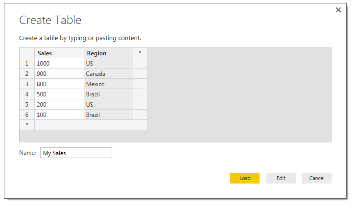
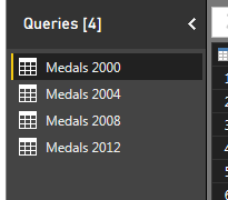
Here’s what happened. I had a PBIX file that had four queries in it, one file for the summer the Olympic metal count for the following years, 2000, 2004, 2008, and 2012.

Olympic Metal Count

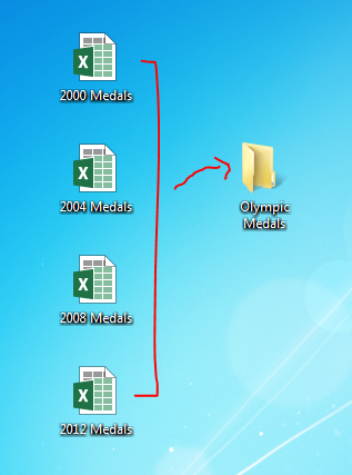
After a bit of working I figured that my desktop screen was going to get to cluttered if I continued to collect Olympic metal data. Thus, I moved my excel files which were my source data into a folder called Olympic Medals.

File Move

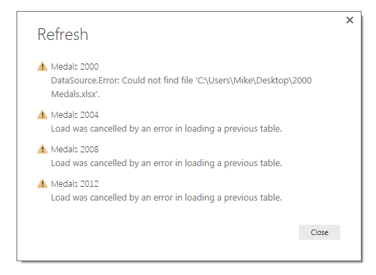
By doing this I broke all the links for all four files. This was discovered when I tried to refresh my queries and noticed that all the queries failed. Power BI gave me a nice little message notifying me that there was a data source error.
```
DataSource.Error: Could not fine the file:
```
Missing File Error

To fix this I had to open the query editor and change each file’s location to the new folder that I just made. Seeing that this is not an efficient use of my time, I decided to spend more time to figure out a way to make a variable that would be my file location for all my queries.

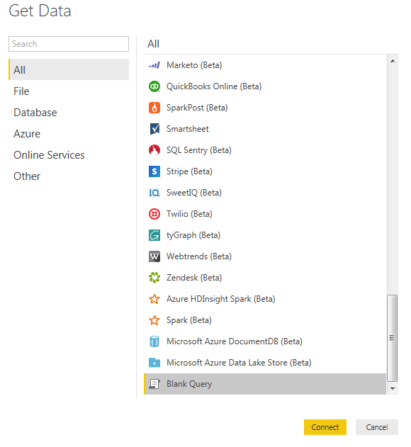
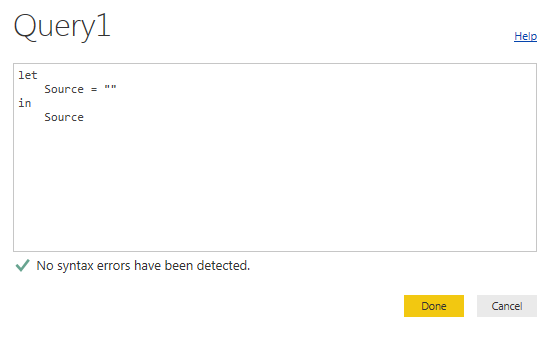
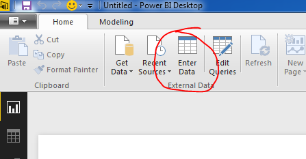
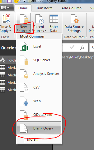
Lets begin by making a new blank query by clicking on the bottom half of the New Source button on the Home ribbon. Then click the item labeled Blank Query.

Start Blank Query

With the new query open type in the file location where you will obtain all your working files. For me my file location was on my desktop, thus the file location is listed below. Rename the new query to Folder.

Folder Query

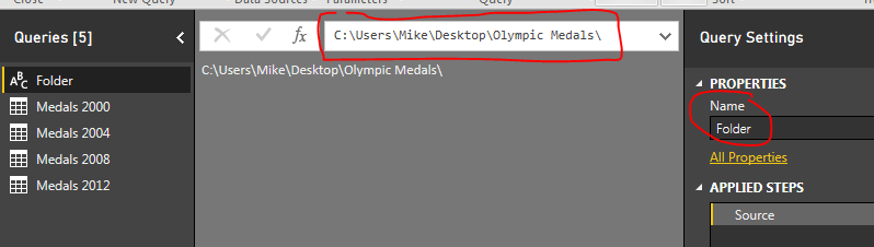
Note: Since we are working on building a file structure for Power BI to load the excel files you will want to be extra careful to add a “\” back slash at the end of the file location.

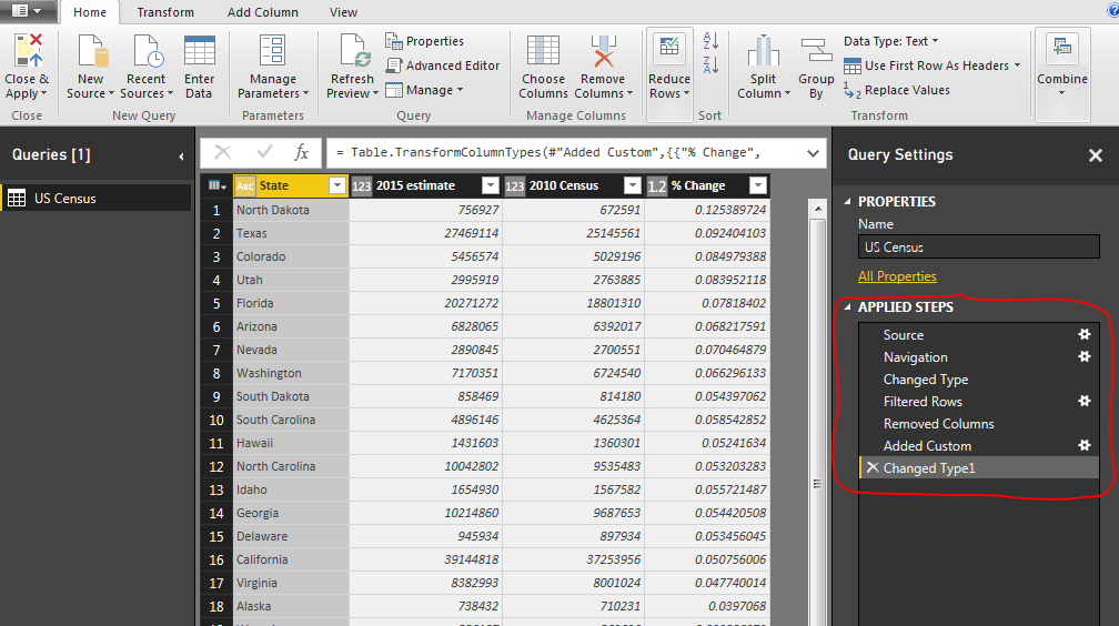
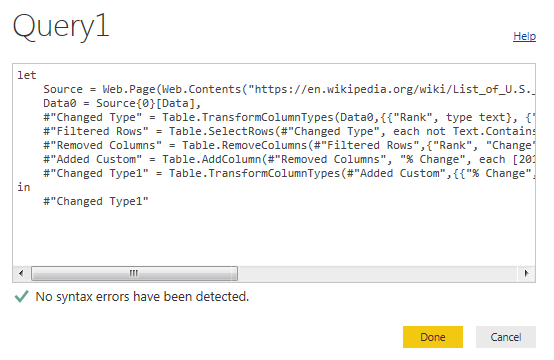
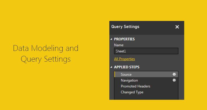
Next on the query for Medals 2000, we click the Source under the applied steps window on the right. This will expose the code in the formula bar at the top of the window.

Select the Source Applied Step

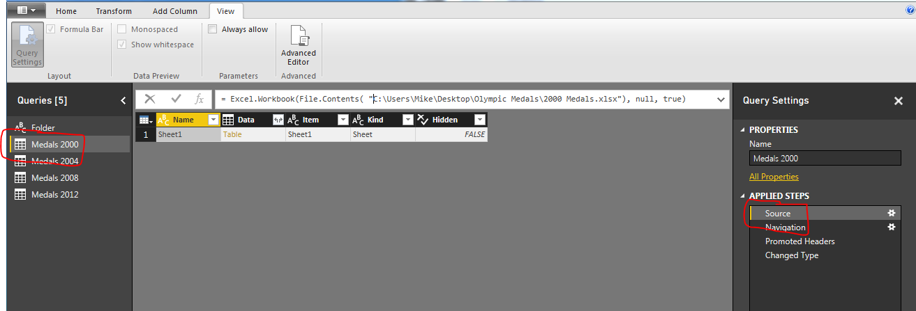
Note: If you don’t see the formula bar as I have illustrated in the image above, you can turn this feature on by click the View ribbon and checking the box next to the words Formula Bar. This will expose the formula bar so you can edit the source step.

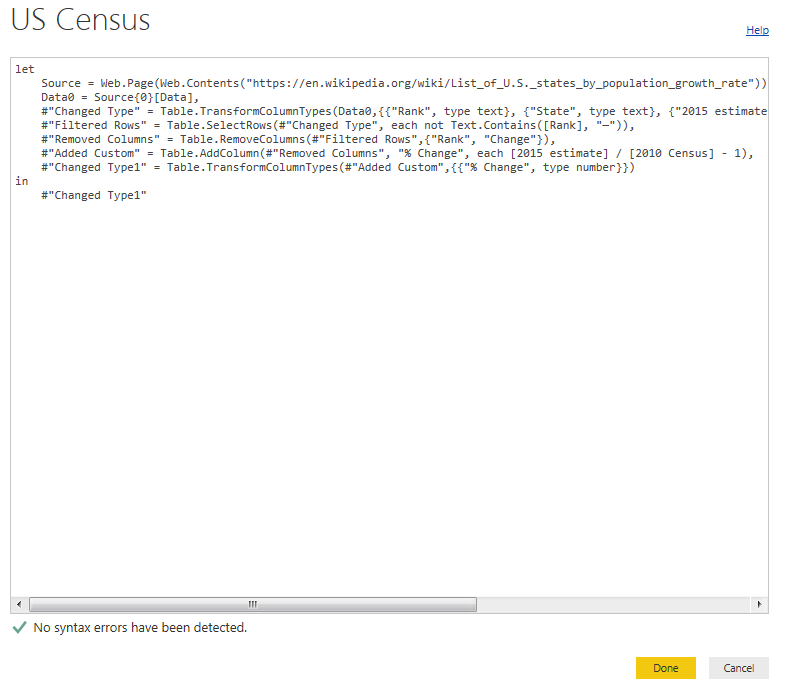
This is where the magic happens. We can now insert our new blank query into this step. Our current file contents looks like the following:
```
= Excel.Workbook(  File.Contents(  "C:\Users\Mike\Desktop\Olympic Medals\2000 Medals.xlsx") ,  null ,  true )
```
Now remove the first part of the file location and make the equation match the following:
```
= Excel.Workbook(  File.Contents(   Folder  &   "2000 Medals.xlsx") ,   null , true )
```
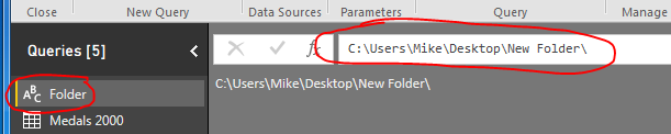
Not only does this shorten our equation, it now uses the folder location we identified earlier and then we can pick up the file name 2000 Medals.xlsx. This makes is very easy to add additional queries with the same steps. Also, if you move your files to a new folder location, you only have to change the Folder query to reflect the new file location. To test this make a new folder on your desktop called New Folder. Move all the Olympic medal files to the new folder. Now in Power BI Desktop press the Refresh on the Home ribbon. This should result in the Data.Source.Error that we saw earlier. To fix this click the Edit Queries on the Home ribbon, select the Folder query and change the file directory to the new folder that you made on your desktop. It should look similar to the following:

New Folder Image

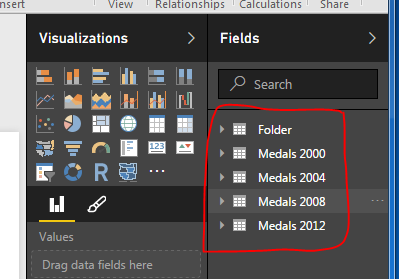
Once you’ve modified the Folder query, click Close & Apply on the Home ribbon and all your queries will now reload. Success!!

New Queries Loaded

Hope this tutorial helps and solves some of the problems when moving data files and storing information for Power BI desktop. Please Share if you like the tutorials. Thanks.
August 4, 2016
Query Editor – Editing M Code

In this tutorial we’ll learn how to copy and paste queries to and from the Query Editor. When your working in Power BI Desktop often you will need to share and model the data before it can be applied to the visual. In my experience you’ll need to add a calculated column or break out a date such as 1/5/2016 into the the Year 2016 or Month 01, components to properly display a visual.

We will start off with from a prior example where we build a shaded region map. The tutorial to create this Power BI Desktop file is located here.

If you want to cheat and download the final PBIX file you can download and open the zipped file here: Regional Filled Map Example

This file was made in Power BI Desktop April 2016 version, 2.34.4372.322, download the latest version from Microsoft Here.

Open the zip file that you downloaded and extract the file inside labeled Regional Filled Map Example. Open the file. Once you’ve opened the file on page 1 of the you see a map of the united states that looks similar to the following.

Opened File with Map

Now we well enter the query editor. Click on the Edit Queries on the Home ribbon. You opened the Query Editor. In this window we shape and model the data so we can properly visualize it on the pages. Couple of things to notice here. Every time you press a button on the ribbon, the query editor generates an Applied Step. Each step writes a line of M code which transforms the data as it is loaded into the computer’s memory. In this case we have (7) seven steps starting at Source and ending with Changed Type1.

Query Editor Revealing Applied Steps

We want to expose the code that is begin generated at every step behind the scenes. Click on the View ribbon and then click on the button called Advanced Editor.

Query Editor – Advanced Editor

Opening this window reveals the M language code that is generating each Applied Step we saw earlier.

Note: some of the steps we saw earlier such as Filtered Rows had a space in it. In the query editor any applied step had a space in the name gets the added #”” around the applied step name. Thus, in the query editor Filter Rows would be #”Filtered Rows”. The hashtag and the quotations define the complete variable. If you changed the name of the applied step to FilteredRows, with no space. In the Advanced Editor you’d only see the step labeled as FilterRows, no hastag or quotations needed.

Now that the M language is revealed you can made modifications to the code. In cases where you want to make a function you would do so in the Advanced Editor. For our example today select all the code and copy it to the clipboard using the keyboard shortcut CTRL+C. Click Done to close the window.

Now lets copy that code into a brand new query. Click the Home ribbon, then click New Source, scroll all the way to the bottom of the list and select Blank Query. Click Connect to start a blank query.

Get Data – Blank Query

A new Query will now open up. Click the View ribbon, then click Advanced Editor. A blank editor window will open.

Blank Query

Paste the code we copied earlier into this window. Now the new Query1 should look like the following:

Paste Code in to Advance Editor

Click Done and the new query will now load. It is that simple, now we have two identical queries.

May 19, 2016
Manually Enter Data
There are often times when you need a small data set in order to make a visual behave exactly how you want it to. This may mean you need a small table to represent a range of numbers or text values.

Here are the Resources for this tutorial:
- Power BI Desktop (I’m using the March 2016 version, 2.33.4337.281) download the latest version from Microsoft Here.
To enter your own data Click the Enter Data button on the Home ribbon.

Enter Data Button

Next you are prompted with the Create Table window. In this window you are given the layout of a unfilled table. To begin entering data you can click in the first cell in Column one and start entering data. By pressing enter a new cell will populate below. You can Rename the column by double clicking the column name. To add a second column you Click on the * symbol next to your existing column. Finally to edit the table name you can type in the desired table name in the Name input box in the bottom left hand portion of the window.

Create Table Window

Finally, you can either to choose to Load the data as is or Edit the data to make additional changes (this can be useful to edit the data types of each column or to populate equations in subsequent columns). For the sake of this tutorial we will simply load the data. Click Load to load the data into the data model.

Now drag over the columns into the page view to begin generating visuals. By default PowerBI makes a table of data to show you the values you just entered.

Visual of Sales Table

Select the table visual (you know it is highlighted when it has the trim boarder as shown above) and Click the Doughnut Visual. This transforms the data into a doughnut, and who doesn’t like a nice data doughnut? Click anywhere in the page to de-select the new doughnut visual. Add a second table by dragging over he Region and Sales columns. We can now see the pretty graphic and the numbers supporting that visual.

Visuals Made with our Custom Data

I bet you didn’t notice that something changed here. Look closely at the data we see now vs. what we entered earlier. Go ahead, scroll up, I’ll wait… Did you catch it?

We now have 5 rows of data but we entered 6 before. That is because the Sales column is a number column and can be aggregated. Look in the fields column and you see there is a little sum symbol in front of the Sales column. This means that this column has a default summarization associated. To see what is the default summarization highlight Sales by clicking on the column name in the grey area. Then Click the ribbon titled Modeling, and there it is in the properties section the Default Summarization is Sum. Every time you use the Sales column it will be summarized in the tables and visuals views. Our visual table shows Brazil with a total sales of 600, because we had two Regions labeled as Brazil 500 and 100.

Now you can click on any of the data points in the doughnut. Notice the table automatically filters down to only show the areas you selected.

Data Filtered to only Brazil

ProTip: you can select multiple selections by holding down CTRL and selecting multiple items in the visual. You can only do this inside of one visual. As soon as you click another visual all filtering will disappear.

Again, I hope you enjoyed this quick tutorial. If you liked it make sure you share it below.
April 13, 2016
Query Settings – Fixing a Missing File
One of the most important concepts to learn within Power BI Desktop is how to build a Data Model.

Note: In simple terms the Data Model is data that is collected from the get data function. In your data model you can build multiple queries. This data is stored in the file. The data storage is very efficient as the data compressed down to approximately a 4:1 ratio. 1000 KB file will compact down to approximately 250 KB when loaded into Power BI. From my current understanding all data is loaded into the memory of the computer. Thus, if you are having performance issues it could be in part due to the RAM of your computer.

As you begin to craft more data models you will learn little tips and tricks along the way to make an efficient Data Model for your visualizations. I have found that the most challenging part of building the data model is structuring the data in a way that will make your selected visual make sense. This may mean you need to add a measure or a calculated column or a ranking to a data set. Alright lets get started.

Here are the Resources for this tutorial:
- Power BI Desktop (I’m using the March 2016 version, 2.33.4337.281) download the latest version from Microsoft Here.
- We are going to work through the Power BI Desktop file that we built in the Loading Excel Files Into Power BI Tutorial. You can follow the link to create the Power BI Desktop (pbix) file in the tutorial. For convenience, the completed file can be downloaded here: Import Excel Tutorial.
I’m going to start off by extracting the Import Excel Tutorial.zip file to my desktop. Once the file has been extracted we can open the containing folder. In this folder there are two files the source data in the excel file and the Power BI Desktop file.

Note: A Power BI Desktop file has a .pbix file format ending.

Open the Import Excel.pbix file. First click the Home ribbon and then click the Refresh button. Most likely there will be an error similar to the following message.

Message box when file can’t be found

This type of message occurs when you refresh a query and the file is missing or can’t be found. This is because when i originally built the Power BI Desktop tutorial the excel file that is supply the information was located on my desktop. This is a common problem when you build connections to local files stored on your computer. If you move a file into a different folder then the connection will break.

To resolve this close the message window by clicking Close. on the Home ribbon click the Edit Queries button. The Query Editor window will be presented. In a large yellow bar in the data view portion of the window (circled in red) is the error message.

Note: Circled in blue is the Query Settings window. This window is the window for all the applied steps to transform the data. You can change the name of the query in the name box. From the view we have selected we can see that the step entitled Changed Type is currently selected (seen circled in blue).

Click the grey button labeled Go To Error which is found in the yellow error box.

Error seen inside Query Editor

Upon clicking the Go To Error button the selection in the Query Settings button to the Source Step. This is where the query has failed. More information about the failure is shown in another yellow error box. This time click Edit Settings in the error box.

Edit Settings in Error window

Now we have the Load Excel file window prompt open. In this window Click Browse, navigate to where you extracted all the files downloaded earlier in the tutorial and select the excel document entitled Book1. Click Open and the new file location will be loaded into the Load Excl Window. Click OK to complete the settings change.

New File Location

Now the data is correctly loaded into the data model. Notice we are still on the step called Source. Take some time to click through each step, Source – Navigation – Promoted Headers – Changed Type. As you click on each step you can see how the data is transforming.

To see the code that is being used to make each step click the View ribbon and check the little box entitled Formula Bar. This will make a formula bar appear. When you click on a step the formula bar will reveal the code needed to complete the selected step.

Toggling on the Formula Bar

We can now see the equation, which is similar to how you would write an equation in excel. The code in the Changed Type step is here:
```
= Table.TransformColumnTypes(#"Promoted Headers",{{"ID", Int64.Type}, {"Sales", Int64.Type}, {"Category", type text}})
```
The equation is using the M language to transform the data. More information on the usage of the M language can be found here.

Note: Couple of pointers about the data shown in the formula. The function is called Table.TranformColumnTypes. The source of the data is a variable called #”Promoted Headers”. The pound sign and the words following in quotations is how the M language passes variables that have a space contained in the language. Since the prior step has the name “Promoted (space) Headers” the program has to add the pound sign and the quotation marks. If there is no space in the naming convention such as “PromotedHeaders” then only the PromotedHeaders would be seen in the code and the pound sign and quotes will be gone. See modify coded when I remove the space from the Promoted Headers applied step.
```
= Table.TransformColumnTypes(PromotedHeaders,{{"ID", Int64.Type}, {"Sales", Int64.Type}, {"Category", type text}})
```
Notice the the pound sign and quotations are missing.

The second part of the formula is an array which has been written out in curly brackets:
```
{
{"ID", Int64.Type}, 
{"Sales", Int64.Type}, 
{"Category", type text}
}
```
I changed the code by adding line returns to make it easier to read. The coded array has beginning bracket and an ending bracket. Each parameter is contained in it’s own curly brackets and separated with a comma. The array is a 2 x 3 array, it has 3 rows and two data points on each row, just like a matrix. The first data point is the column name. In the first row the column that is being address is called ID. The data transformation parameter is called Int64.Type. This means that the data is an integer type 64 bit. This repeats for each row until all parameters have been addressed.

So there you go, we have opened up a query repaired it and learned a little about the formula bar.

As a side note, as you build queries each button press that you make on the various ribbons in the Query Editor will make a minimum of one step the in the Query Editor.

Hope you enjoyed this short tutorial about the Query Editor. Make sure you share below if you liked it.
April 11, 2016