In October of 2019 Power BI released a new file type, PBIDS. The Power BI Desktop Source (PBIDS) file is a JSON object file that aids users connecting to data sources. In true PowerBI.Tips fashion we have of course, made a tool for that.
Introducing Connections
Today we release the new tool called Connections. It can be found at https://connections.powerbi.tips/ . With this tool you can use our predefined templates or customize one of your own file. To learn more about this sweet sweet JSON editing tool check out the following YouTube Video:
Technical Details
For more information on the Power BI Desktop Source file check out these links:
If you like the content from PowerBI.Tips please follow us on all the social outlets. Stay up to date on all the latest features and free tutorials. Subscribe to our YouTube Channel. Or follow us on the social channels, Twitter and LinkedIn where we will post all the announcements for new tutorials and content.
Introducing our PowerBI.tips SWAG store. Check out all the fun PowerBI.tips clothing and products:
This post will walk through how to pull daily stock price from Yahoo! Finance, then transform the data using a technique called a query branch. It will be completed all in the Power Query Editor. We will convert this to a function to reuse on any stock we want.
There are many API to pull stock information that get historical stock prices. Many come with a cost to get this information in a decent format. The technique described here is free but will require some data transformations to get the data in a usable format. The purpose is to explore parameters, web URLs and query branches to design a usable function. If you’re just interested in pulling stock information, skip to the end to grab the M code – just make sure you read the performance considerations.
Note: The content in this blog was first presented at the Power Platform Summit North America on October 18th, 2019.
Getting Started
This blog will use parameters to create functions in Power Query. Some experience using Power Query editor may be helpful, specifically: – Knowledge of tools such as merge and append queries – Familiar with query steps and the formula bar
For a detailed look at parameters or if you need to brush up, check out this post on parameters.
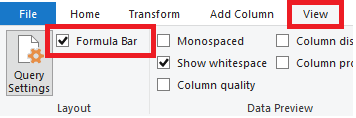
Before starting, you will need to ensure the formula bar in the query editor is open.
Open the Power Query Editor by Clicking the Edit Queries on the Home ribbon of Power BI desktop. Then, go to the View ribbon in the Query Editor and make sure the check box for Formula Bar is turned on.
Create the Parameter
First, Create a Parameter. This is a value that we can change and feed into our query, in this case the stock symbol.
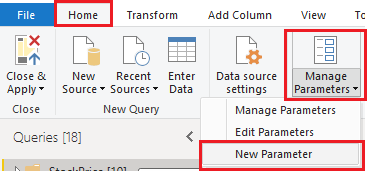
In the power query window, under the Home ribbon, Click the bottom half of the Manage Parameters button. From the drop down Select the option New Parameter.
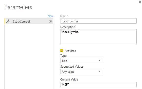
In the Name section, enter the text StockSymbol (without spaces – this makes it much easier to reference later). Give it a description if you like. If you share this report other people can read the description to understand what the parameter is being used for. Change the Type field to Text. Enter MSFT in the Current Value input box. By the way, MSFT is the stock symbol for Microsoft.
Making the Query
Now we have set up a parameter, we can use it to pull in some data. The data source is going to be a web URL. In Power Query editor window, Click the Home ribbon and the button Get Data. Select the item Web in the drop down. In the popup dialogue, Click on the button labeled Advanced.
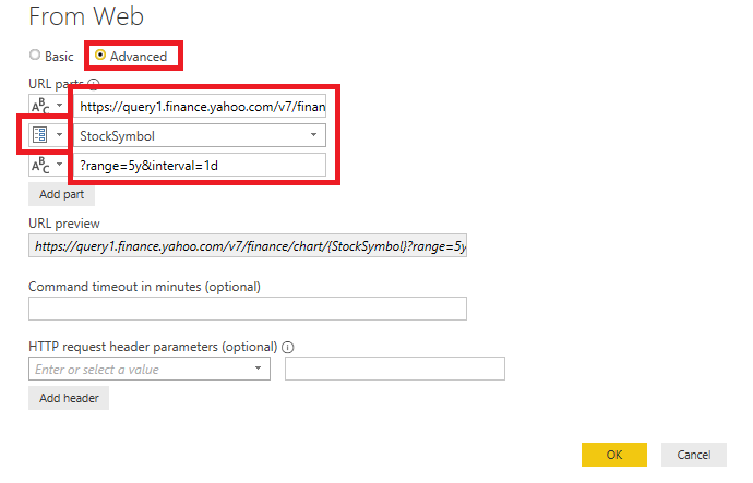
You’ll notice this brings up a dialog called URL Parts. This allows us to break down the URL into parts. We can easily change individual parts of the URL using this dialog. It will then concatenate it all back together in the order it is entered. Our URL to connect to Yahoo! for a single stock will be split into three parts.
The base URL, which points us to Yahoo! Finance website and the correct data
The stock symbol, in this case will be our parameter
Our other settings (range and interval). These could also be changed in Power BI with a parameter, but we do not want to for this example
In the open dialogue box, first Click the button Add part. This will add a new box. Locate the first window and Enter part 1 of the URL. In the second box, Change the abc symbol to a parameter. Make sure Stock Symbol is selected. In the third box, enter part 3 of the URL. We’re setting the range to 5y (5 years of data) and the interval to 1d (daily). You can change these if you want at a later time.
Note: It is important to remember that Stock Symbol is a parameter – change the symbol to parameter and select from the drop down. Do not type Stock Symbol into the box.
Now Hit the button labeled OK. The request will be sent and returned to us in a JSON format.
Rename the query Stock Value. You can edit the name above the Applied Steps section on the right.
Making the Query Branch
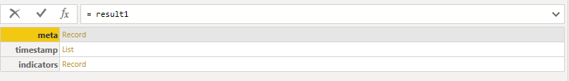
The data returned is a little messy and not in the best format. We need to drill down and pull out the appropriate bits of information. Start by drilling down to the correct information. To drill down, Click the underlinedresult part in the following order: Chart: Record Result: List 1: Record
Your screen should look like the image below. If it doesn’t, simply delete the navigation step and start again.
Here, we are presented with three options of paths to drill down further:
Meta: holds some info about the stock, as well as the timeframe and granularity we chose Timestamp: a list of the dates in the range we selected Indicators: this holds the price information of stock
Right now, the dates and the price are in two different
lists. The price information is another layer down than the dates which makes
this more complicated. Extracting these individually would result in a list of
random prices and a big list of dates – not helpful if these two pieces of
information are not together.
To solve, we will create a Query Branch. The branch will split our query at this step into two paths. One will retrieve the dates, the other the prices. Then we will merge these branches back together to get the dates and prices in the same table.
To start this branch Right Click on the Navigation Step, then Select the option in the drop-down menu Insert Step After. This will reference the previous step and show the same data. Our newly created set is the start of the branch. Rename this new step StartBranch.
Note: the reason for this reference is that the “Navigation” step is not really a step at all. It is actually a collection of steps that Power Query editor groups together. You cannot reference “Navigation”, which will be needed later. You’ll see you cannot rename the Navigation step and if you open the advanced editor you can see the breakdown of individual steps. Another option is two perform any action after the Source step, before you drill down. This will cause Power Query to list each drill down step individually.
Branch 1: Dates
Our first branch we
will pull the dates.
Click on timestamp: List. This will drill down to a list of dates, but they are stored in a UNIX format. UNIX date format is the number of seconds past January 1, 1970 (midnight UTC/GMT), not counting leap seconds. Converting this is quite easy but will take a couple of steps.
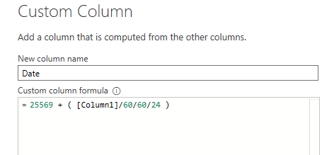
First convert the list to a table so we can perform transformations. Click on Transform ribbon. Select the button To Table. Next, under the Add Column ribbon Click the button Custom Column. Change the name to Date and use the following formula in the formula window:
25569 + ( [Column1]/60/60/24 )
Then Select the Date column. Click the Transform ribbon. Under the Data section, Select the Date format. Note: do not select the Date/Time.
Now we have the date but need to preserve its order. This can be solved by adding an index. Go to the Add Column ribbon, Click the little Drop down on the right half of the Index Column button. Select the option From 0 from the drop down menu. Remove the column labeled Column1, as it is not needed anymore. To do this, Right Click on Column1 and select the option Remove from the drop down menu.
This finishes the branch for the dates. Rename this step EndBranchDate by Right Clicking the step in the APPLIED STEPS and Clicking rename.
Branch 2: Prices
Now we need to get the information for the stock prices. Right ClickEndDateBranch and Click the option Insert Step After to add the start of the branch. By checking the formula, we can see it says
=EndBranchDate
This step is doing is referencing the step before it, EndBranchDate. It is duplicating the output of this step. We need to get back to the StartBranch step in order to start the second branch. Change the value in the formula bar from = EndBranchDate to = StartBranch.
This now loads us back to this step to drill down to the stock prices. We will use the adjusted close – this is the stock price at the end of the day after adjusting for dividends. Here we need to drill down to this information, by drilling in the following order:
Indicators: Record adjclose: List 1: Record adjclose: List
Next, Covert our list to a Table. see above for this step. Here we have the list of prices and again need to preserve the order with an index column. Go to the ribbon labeled Add Column. Click the Index Column and select From 0 in the drop down.
This is the end of this step, so Rename it EndBranchPrice.
To summarize the query so far:
Pulled the information for a MSFT stock for 5 years on a daily basis.
Drilled down to the dates, converted them to a better format and added an index to preserve order.
Revert to an earlier step.
Drilled down to the daily prices and added an index column.
Merging the Branches
This leaves two separate tables, but it is only possible to output one of these results. We will need to add a final step to merge these two branches into one table.
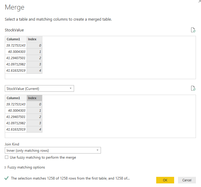
On the Home Ribbon, Click the drop down arrow on the Merge Queries button. Then Select the option Merge Queries. This brings up the merge screen. Merge the query with itself. On the bottom half of the merge, Select StockValue (current). Click on the Index column for both top and bottom.
Clicking OK, will merge the data to itself. This is the formula in the formula bar:
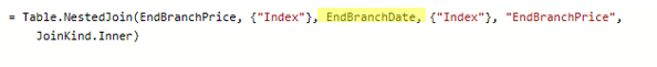
This step uses the Table.NestedJoin formula, which has 6 arguments filled in:
Table.NestedJoin(table1 as table, key1 as any, table2 as any, key2 as any, newColumnName as text, optional joinKind )
In our example, table1 and table2 is the same (EndBranchPrice). This makes sense as we joined it to itself. You will notice that when joining from the same query, the table argument references a step in that query (EndBranchPrice). We really want to join EndBranchPrice to EndBranchDate. We can simply change the second table in the formula bar to EndBranchDate:
Change:
To:
Now, we are joining the EndBranchPrice to the step EndBranchDate. These both have a column named index that we added, which will join our data in the correct order.
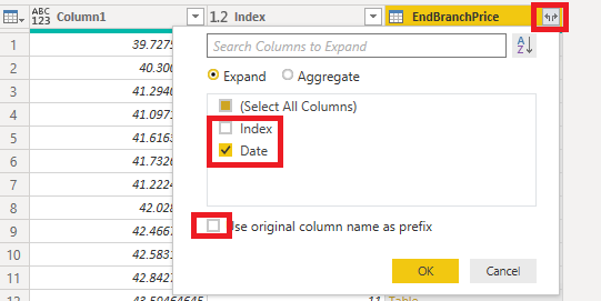
Expand the merged table by Clicking the Expand button on the column name. The settings will just Select the Date and Deselect the option to Use original column name as prefix.
Remove the index column as it is not need this anymore. That completes our query with the branch.
Enabling Publish to the Service
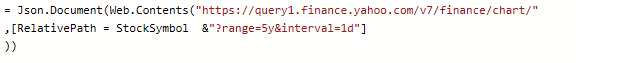
If we want to publish this to the service (app.powerbi.com), we will need to make a small edit to our URL. The service will not allow parameters in the base URL. To get around this, we can split our URL using an option in Web.Contents called RelativePath. After Clicking on the Source in the applied steps window, Edit the URL as follows:
From:
To:
Make sure the brackets are correct. Here is the code you can copy and paste into the formula bar:
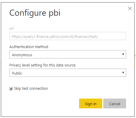
Now we have changed the URL, we need to make a change to the settings. This is because Power BI will try and check the base URL (https://query1.finance.yahoo.com/v8/finance/chart) before it runs the query and adds the second part in RelativePath. This isn’t a valid URL on its own, so it will fail.
To do this, publish the report to the service, and Navigate to the dataset settings. This is found in the service by Clicking the ellipsis in the top right, then the option called Settings in the drop down.
You should be in the tab called Datasets. Then Navigate to the published dataset. Under the option titled Data source credentials, next to Web, Click the option to Edit Credentials. Make sure to check the option to Skip connection test.
This query uses a parameter which enables us to can convert it to a function. To do this, right click on the query in the Queries pane on the left and select make function.
Now we have a function where we can input any stock symbol and return a list of daily prices. To check multiple stocks, you can add your function to any list of stock symbols. This can be found in Add Column ribbon. Then Clicking the button Invoke Custom Function. This will return a table for each row. Before expanding, it is important to handle errors, otherwise it could break the query. One option is to Right Click the column header, and select the Replace Errors option, and Type the text null.
Performance Considerations
While this query will quickly return single stocks, adding multiple stock will send a different query for each stock. Make sure you design the correct solution to what you are trying to achieve, and check out this article on API considerations.
Final Result
For those who like M code, here is the final function. You can copy and paste this directly into the advanced editor (See this article on how to do this).
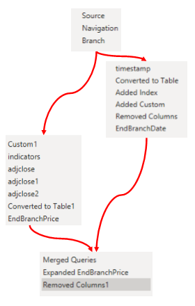
Visually splitting the steps, the query can be visualized like this:
If you like the content from PowerBI.Tips please follow us on all the social outlets to stay up to date on all the latest features and free tutorials. Subscribe to our YouTube Channel. Or follow us on the social channels, Twitter and LinkedIn where we will post all the announcements for new tutorials and content.
Introducing our PowerBI.tips SWAG store. Check out all the fun PowerBI.tips clothing and products:
We are starting today off with a fun chart. We will be making a filled donut chart. Typically, I don’t use donut charts but in this case I think we have a good reason, and it’s delicious…
The data being used in this visual varies from o to 100%. This could be something like a test score or a compliance number. Thus, we will be using the donut chart to represent a completion of 100% or some variant below.
Video on how to build this chart.
During this video we used a couple measures. They are the following:
Measures
Average Product Score = AVERAGE( 'Product Scores'[Score] ) / 100
Average Product Score Inverse = 1 - [Average Product Score]
Where the value of the Score comes from the Product Scores table. The Score column ranges from 0 to 100%. If you like this visual and want to download a sample file visit my GitHub page.
If you like the content from PowerBI.Tips please follow us on all the social outlets. Stay up to date on all the latest features and free tutorials. Subscribe to our YouTube Channel. Or follow us on the social channels, Twitter and LinkedIn where we will post all the announcements for new tutorials and content.
Introducing our PowerBI.tips SWAG store. Check out all the fun PowerBI.tips clothing and products:
As report authors we sometimes get caught up in how easy it is to create a report and provide value to the business. Each report is an opportunity to make a big contribution to the organization. Power BI makes it easier than ever to turn many of those reports around quickly. This is a good thing of course. But, sometimes we can get caught up in the madness of turning out another report with only a flash of recall that we could have used the same or similar model done in a different report. The internal monologue kicks in.
“Pffft! Re-use a model, that is way to much work! Why do that?, when we can just create a copy of the PBIX (Desktop file) and have two models to manage with the two reports for the same business area! That sounds like fun!”
Hmm… Or does this actually sound awfully similar to the challenges one might face with sprawling Excel solution. Where variants of logic are buried in different files. Only the composer knows how to bring order from the chaos. Might I suggest that we spare ourselves that sort of pain. Just learn how we can easily leverage our already hard fought model work. Avoid tedious updates without having to over complicate our nirvana of sticking to the business world, but how would we do that?
The Answer
Power BI datasets. Power BI datasets allow us to re-use our model across multiple reports. This simplifies and speeds up future report authoring. Also this gives us the building blocks for sharing that dataset to a wider audience.
How do we create one?
Technically, we’ve likely already created many. You see, when we publish a Power BI report, we publish a dataset along with it. This dataset is stored in the Power BI Service, and our deployed report relies on it now. But the connector “Power BI datasets” allows us to connect directly to any of these datasets that we have permission to edit. This means that we have the ability to extend a single model across multiple reports without the need of standing up a separate Analysis Services server anywhere. This is a big deal, this allows the everyday business user to leverage a reusable model. A single change or update to a calculation can update multiple reports at the same time. One measure or calculation addition can be done in one place instead of many.
All we need to do to create a dataset that we can connect to is publish a PBIX file that contains data. I’ve adopted a practice recently and rather than generating my first report and reusing that model, I now upload a PBIX file that ONLY contains the model and I name it something like “Sales-Model”. Now I have an object that I’ll know serves the purpose of just being a model instead of a report. This makes it easier from a trace-ability standpoint when looking at the related objects in the Service or selecting it from my list of options when choosing my dataset.
How do we use one?
Using the Power BI dataset is one of the most
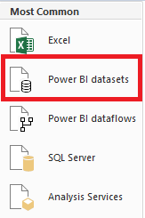
straightforward connections in Power BI. Selecting Get Data -> “Power BI
datasets”
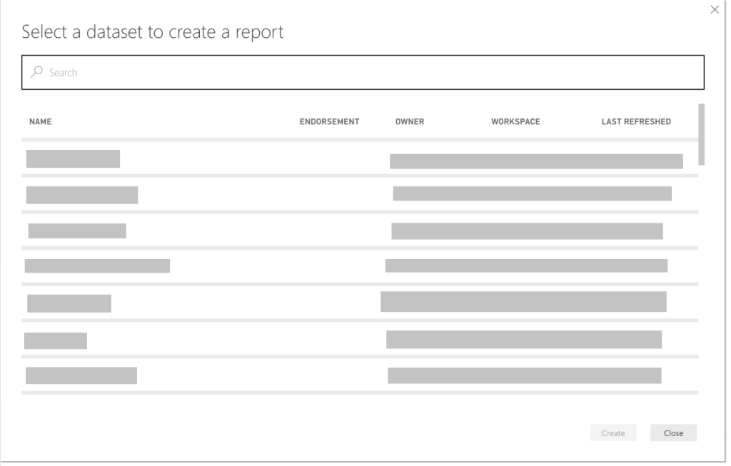
This brings up the menu of all the datasets in the Power BI Service. The list that is shown are the datasets that our user account has access to use. The great thing about these datasets are we now have the ability to connect to and use a dataset from a different workspace provided we have permissions to edit them. This feature is called a Shared Dataset. Select the dataset and your report is automatically connected to dataset.
Now, what we’ll notice here is that using this feature automatically pulls in a model for us and we can start building our report. This data source connection behaves exactly the same as if we created our own “live” connection to an Analysis Services instance we would set up. Probably not shocking to any reader here. But, that is exactly what is happening in this case as well. We get the benefit of Microsoft handling all that painful work for us while we reap the benefits of a streamlined process.
As with any “easy button” solution, there are pro’s and con’s. What I mean is that in our new reports we do have easy access to the model. Now you can start building reports immediately. We don’t have the ability to modify the model or the ETL processes. If we want to edit then we need to go back to the original dataset to make those changes.
But the minor inconvenience of having 2 PBIX files open if we need to in order to make updates to the model is trivial compared to being able to connect many reports to that single model. The live connection does still allow the report author the ability to create measures. So, if there are measures that are only suited to our report and not the overall model we still have the ability to add them.
Once we’ve completed
our report, we just publish as we normally would, only this time the dataset is
already out in the Service and only our report is published. There are so many
things we can now do to share that dataset, but we’ll leave that to another
article.
If you’ve never used this method before, I would highly encourage you to try it out. Any time you can save yourself now with reducing the number of models you maintain, the faster you can produce more reports. You now spend less time maintaining all the reports you are publishing.
Happy report building!
If you like the content from PowerBI.Tips, please follow us on all the social outlets to stay up to date on all the latest features and free tutorials. Subscribe to our YouTube Channel, and follow us on Twitter where we will post all the announcements for new tutorials and content. Alternatively, you can catch us on LinkedIn (Seth) LinkedIn (Mike) where we will post all the announcements for new tutorials and content.
As always, you’ll find the coolest PowerBI.tips SWAG in our store. Check out all the fun PowerBI.tips clothing and products:
This post will answer how to sort a measure that returns text values to a custom order, without affecting other columns. It will utilize the DAX functions of REPT() and UNICHAR(8203) – a Zero width space.
The requirements
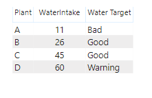
I’ve been working at a florist! In this example, I have been in charge of looking after four plants, named A, B, C and D. The florist owner is a big Power BI fan, and asked me to measure how much water I have been giving them a day to put in a report. They need at least 20ml to survive, but over 50ml will stop them growing as well.
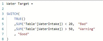
Create a table with the flowing: The flowers get under 20 ml, label as Bad. When the flowers get 20 – 50 ml, label as Good. Finally, if the flowers receive over 50 ml, label as Warning. I’ve been asked to show them in order of Bad, Warning then Good. This is vital so the plants needing attention are at the top of the table.
Creating the table
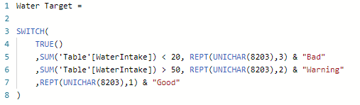
Here is the measure I create:
Adding this to a table:
Now comes the question, how can I order this to put Bad and Warning together? If I order by Water Target measure, this will be alphabetical. Sorting by WaterIntake can not give me the correct order either. One option would be to make a conditional column and use the “Sort by Column”. However, this may be a complicated calculation, especially on more complex measures. In addition it will sort every visual by this column, when I only want to sort in this one table.
Creating the custom sort
My solution? Make use of the UNICHAR() function. For those unaware of this function, UNICHAR() can return characters based on their UNICODE number. This can include more text characters not included on the standard keyboard.
A character that can help is UNICHAR(8203). This is a “Zero width space”. This is a space that has not width, so it is essentially invisible and will not be visible in the measure. The Zero width space is still recognized as a character by DAX. Spaces come before any letter in the alphabet. Two spaces comes before one, and so on.
The second function I will utilize is REPT(). REPT() or replicate, simply repeats text multiple times. It takes two arguments, the text and the times to repeat.
For example: REPT( "Hi", 3 ) will return the text "HiHiHi"
To change the sort order, I will repeat the Zero width space in front of the text. The text I want to appear first will have the space repeated the most amount of times. This will put it first in an alphabetical list. I will use the & symbol to concatenate the Zero width spaces and the text.
Now, “Bad” has the Zero width space repeated three times in front of it. This now puts it first in an alphabetical list. Warning has the Zero width space repeated twice, putting it second. “Good” has it once putting it third.
Applying the sort
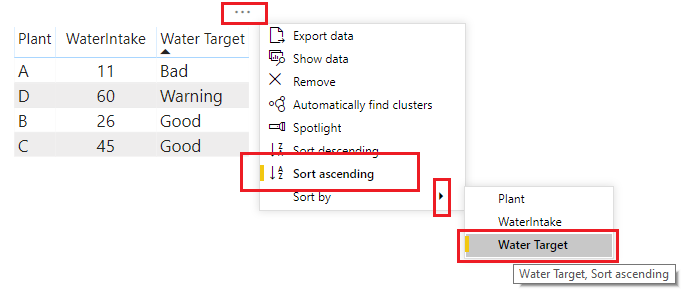
Now I can arrange my table by Water Target (alphabetical), in an ascending order:
And success! I’ve added a custom sort to my text measure, without making any other measures or columns.
If you like the content from PowerBI.Tips please follow us on all the social outlets to stay up to date on all the latest features and free tutorials. Subscribe to our YouTube Channel. Or follow us on the social channels, Twitter and LinkedIn where we will post all the announcements for new tutorials and content.
Introducing our PowerBI.tips SWAG store. Check out all the fun PowerBI.tips clothing and products:
The release of grouping visuals was an extremely welcomed
feature. As one who builds lots of reports grouping elements together is
essential to stay organized and to increase report building speed. Since I’ve
been using this great new, I found an interesting design element to style
groupings for reporting impact. The grouped visuals feature enables a new
property, background color. This can be
applied for the entire group of visuals.
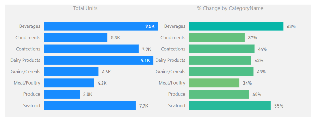
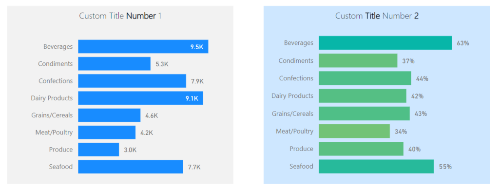
See the following example of setting a background around two
visuals.
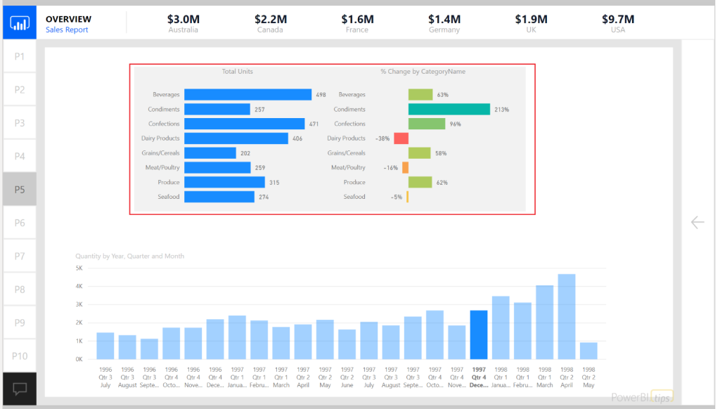
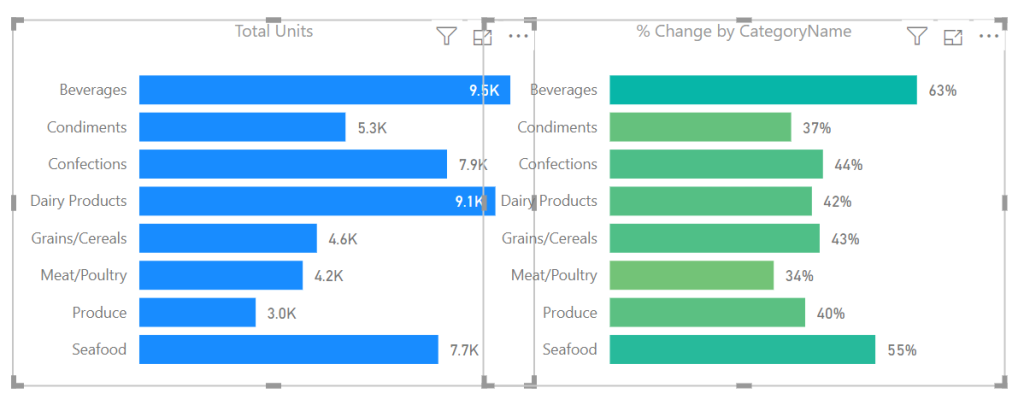
In this example the intent is to show the user that these
two visuals are related. The graph on the left shows the number of units sold
for a selected time period. The bar chart on the right shows the relative sales
over time represented as a percent change. This illustrates the principle of
position and direction. The number of units sold is what happened right now. It
is my place in time with respect to sales. However, this does not show any
context to performance. The percent change provides the directional context. Since the position and direction are an
important insight as a paired visual, we use the grouping to visually bind the
two.
For those who have done some research around design
principals inevitably you will stumble across the Gestalt
Principals of design. Grouping
visuals with a common background falls into the Law of Common Region or Law of
Proximity.
Alright let’s walk through how to use grouping with
backgrounds colors.
Once you have created the visuals which will be grouped together;
select each visual by holding CTRL and Selecting each
visual.
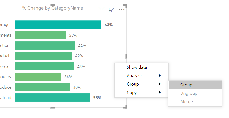
Right Click on one of the visuals and select the menu
item labeled Group, in the flyout menu select the option called Group.
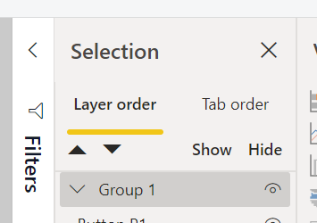
A grouped element will be created in the Selection Pane.
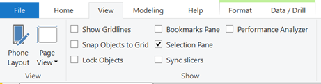
Note: If you don’t see the Selection Pane, you will need
to turn this on. The setting to turn the
Selection Pane is found in the View ribbon with the check box for Selection
Pane. See below for reference.
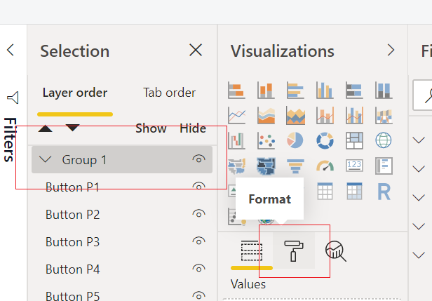
With the newly created group being selected, Click on
the Paint Roller (Format) icon in the Visualizations Pane.
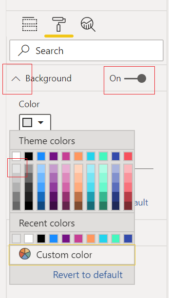
Expand the property section called Background.
Toggle the background to be On and select a Color from the
drop-down menu. For this example, I
selected the very first shade of grey in the first column of colors.
The final product will be a grouped arrangement of visuals
with a shaded background.
To extend this idea further we can take the same approach
when working with Text boxes and Visuals.
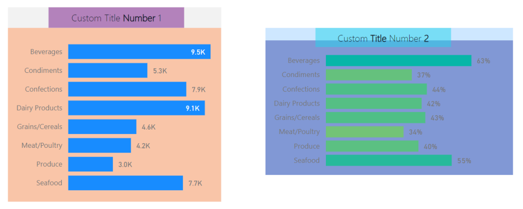
Often, I find I need more style for applying a Text box or header to a
visual. In these cases, I will use two
visual elements to create one visual.
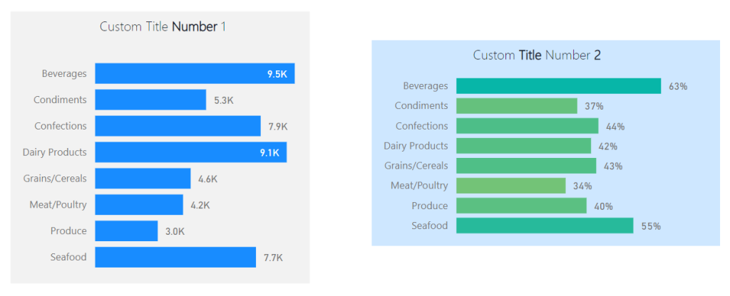
See this example of two visuals with custom titles created with a
textbox.
Note: Backgrounds are colored differently to illustrate
that each background for the grouped visuals is different.
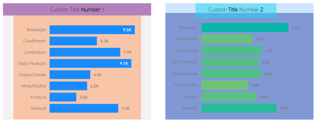
While this meets the need the boxes are not identical in
size. This violates yet another Gestalt
Principle, symmetry. The bounding
regions of the elements inside the grouping define the outer perimeter of the
background shading. Knowing this we can
modify the visuals within the groups to provide a symmetrical background shape.
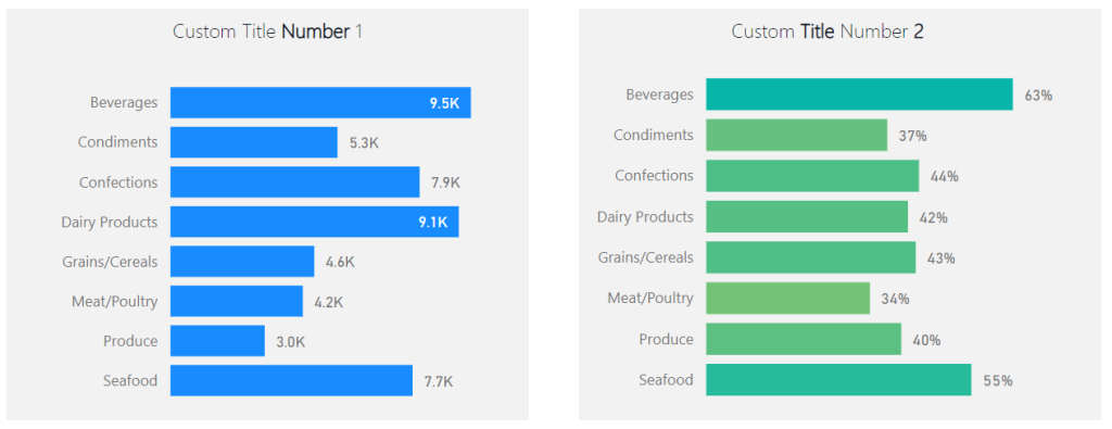
Here are the same before and after images with each visual
object colored to see the adjustments in size for each visual type. This creates the proper background
sizes.
Before:
After:
The visual on the left required an increase of the text box
at the top to get the desired width of the background shape. By contrast the visual on the right required
an extension of the bar chart in length to acquire the desired length of the
background. The result provides a
symmetric view of both visual groups.
If you like the content from PowerBI.Tips please follow us on all the social outlets. Stay up to date on all the latest features and free tutorials. Subscribe to our YouTube Channel. Or follow us on the social channels, Twitter and LinkedIn where we will post all the announcements for new tutorials and content.
Introducing our PowerBI.tips SWAG store. Check out all the fun PowerBI.tips clothing and products:
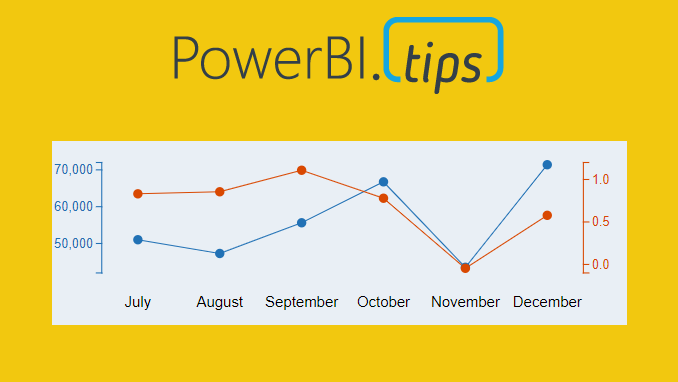
Ever need two different scales on the Y-Axis of a line chart? If so, then this tutorial is for you. While creating a dual y-axis line chart is pretty common in excel, it is not as easy in power BI. The only standard chart that comes with Power BI Desktop that enables dual y-axis is the Column and line combo chart types.
For this particular visual I needed to show correlation between two time series with different Y-axis scales. The Y-axis on the left of the chart had data elements in the thousands, but the right side needed percentages. The tutorial below illustrates how to accomplish by building a custom visual using the Charts.PowerBI.Tips tool.
Video Tutorial
note: there are a bunch of really good custom visuals that can be downloaded from the Microsoft App Source store. However, this article will not review all third party visuals that are able to produce a dual Y-axis line chart.
Source files
All files used to create this visual are located here on GitHub.
Layout file
The file used in this tutorial was a derivation of the Sunset layout from PowerBI.Tips. If you like this file, you can download it here:
If you like the content from PowerBI.Tips please follow us on all the social outlets. Stay up to date on all the latest features and free tutorials. Subscribe to our YouTube Channel. Or follow us on the social channels, Twitter and LinkedIn where we will post all the announcements for new tutorials and content.
Introducing our PowerBI.tips SWAG store. Check out all the fun PowerBI.tips clothing and products:
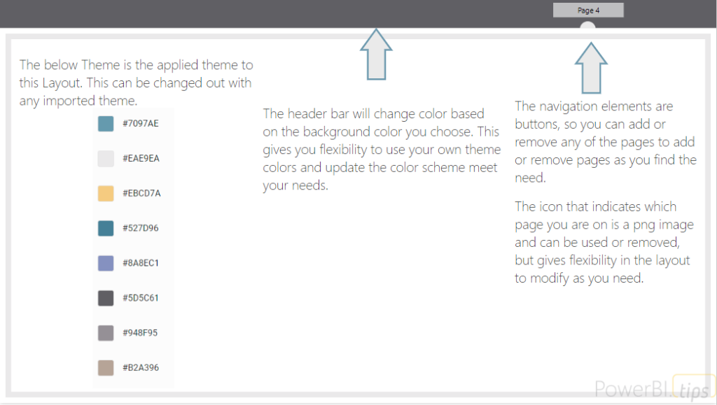
This layout continues to deliver fantastic visual guides to make your reports look top notch. This layout utilizes buttons for navigation without locking in the position in the layout background. We also really like how this layout uses the theme templates to change the background header color to anything you would want. The semi-circle that indicates which page you are on is a free form image and can be changed around if you want to re-arrange the pages. Our branded layout gives you 5 pages of fun, while our unbranded version throws in 10 pages and includes all 10 background .png image files to make your report building even easier.
Features of this report
Free documentation provided by PowerBI.Tips included on the Report Features page
10 pages of different layouts – Unbranded
5 pages with navigation built with buttons in the report (Easily swap out a different background)
10 PNG images of all the backgrounds to use in this report or others – Unbranded
Navigation dot – included icon image for complete flexibility
Customizable top ribbon (color of buttons and background header are can be altered with themes)
No PowerBI.Tips Branding on any of the main report pages – Unbranded
One – Capabilities
Get a feel for all the page layouts and interactions available in this report by using the below example we’ve embedded via Power BI.
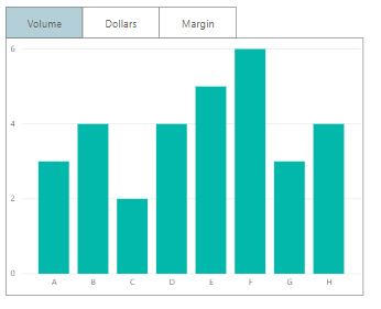
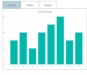
Sometimes, we want the users to see different metrics, but
do not want to take up too much space on our page. The scenario we are going to
walk through is how to build just one visual (in this case a bar graph). It
will include a toggle that allows the user to select their desired calculation,
either the sum of Volume, Dollars or Margin.
Final Solution
With buttons, we can change specific visuals on a page. Recently,
with the release of conditional formatting on titles and backgrounds, we have
some new methods to make this easier for the report author and cleaner for the
report consumer.
The Build
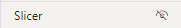
Before we start, turn on the selection pane and bookmark
pane. They can be turned on by clicking on the View ribbon and checking the
correct boxes.
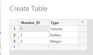
First, we’re going to create our control table. This
will be a disassociated table. This table should not have any relationships to
any of the other tables in our model. We just need to enter a numeric ID and a
description of what we want. Click on
the Enter Data button found on the Home ribbon. Enter the
following data as shown. Click the OK button to close the Create
Table dialog box.
Now that’s set up, we can write our measure. This measure will see what is selected in the Number_ID column of our control table, then return the appropriate calculation. Use a switch statement to select the correct calculation. Create the following measure:
Note: See there is a default value listed in the switch
statement. The default calculation means that if nothing is selected, SUM(
Sales[Volume] ) will be returned. The default value is represented by the last
property in the switch statement.
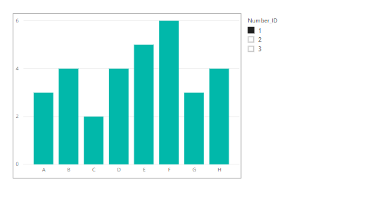
Time to set up our visual. Add a bar graph with Category on the
axis and the new measure, Selected Calculation, in the values
fields. Then add a slicer for the Number_ID column. The Number_ID
column comes from the control table we added earlier.
Switching the slicer can now change the graph to show the
different calculations.
The next stage is to add three buttons to the top of the
graph. In the Home tab of the ribbon, click Buttons and select Blank. Make sure
the outline colors and outline width match on all objects, Buttons and chart
outline.
Tip: Make sure you label your buttons in the Selection Pane. The selection pane can be turned on by clicking on the View ribbon and checking the box labeled Selection Pane. To Change the name of the button, double click the name listed in the Selection Pane. Giving a title (such as Button_Volume) will make it easily to see what visual items are on the page.
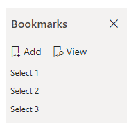
After this, it’s time to add the bookmarks.
The bookmark pane can be turned on by clicking on the
View ribbon and checking the box labeled Bookmark Pane.
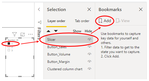
Step 1:
Select a value of 1
in the Number_ID slicer.
Select the slicer (and only the slicer) in the
Selection pane.
Click “Add Bookmark” in the Bookmarks pane.
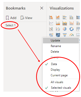
Step 2:
In the Bookmarks pane, right click the bookmark and rename it to Select 1.
Right click again, and untick “Display” and “Current Page”. Select “Selected Visuals”.
Now repeat step 1 and step 2, but do so with the values of 2 and 3 from Number_ID
slicer. Name these bookmarks Select 2 and Select 3. You should finish with
three bookmarks, each that filters Number_ID to a different value. You
can test the bookmarks by clicking on them once in the bookmark pane.
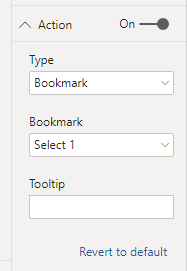
On Button_Volume, assign the Select 1 bookmark (as Number_ID
1 refers to volume). To do this, click on Button_Volume in the selection pane.
In the visualizations pane for this button, go to the property named “Action”.
Turn it on, change the type to bookmark, and choose Select 1 in the dropdown.
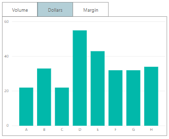
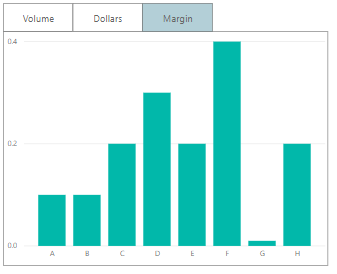
Repeat for Button_Dollars and assign Select 2. Then
for Button_Margin and assign Select 3. Now the buttons can change the
graph, but it’s a bit hard to see what is selected.
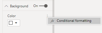
Add Conditional Formatting
This is where conditional formatting can help us! Select Button_Volume
in the selection pane. Then in the visualizations pane, turn on the background
property, select the ellipsis and click conditional formatting
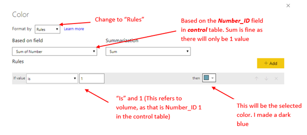
Here’s the settings we want:
This is going to apply a rule if the Number_ID selected is 1, to give the button a blue background. As there are no other rules, any other number selected will default to the white.
Now, apply the same steps to the other two buttons, but make
the rule “If value is 2” for Dollars, and “If
value is 3” for Margin.
To tidy up, hide the slicer and turn the visual headers of all buttons off. You can click on the eye next to the slicer in the selection pane to hide it.
Turn the visual headers off by clicking the button, then in
the visualizations pane.
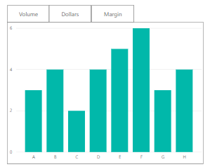
Great! Now the tab shows the selected button and correct
measure:
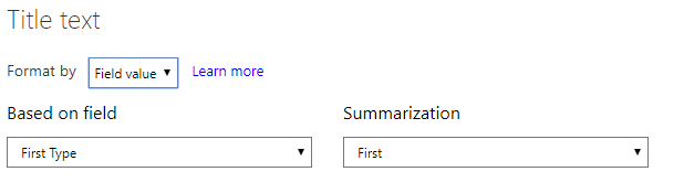
To make it even clearer, apply conditional formatting to the
title of the graph. On the graph, open conditional formatting. Set it to field
value and use the type field in the control panel.
Using this control table allows for greater flexibility. We can add more calculations, easily edit them or even sync across pages, all without having to re-record any bookmarks.
If you like the content from PowerBI.Tips please follow us on all the social outlets to stay up to date on all the latest features and free tutorials. Subscribe to our YouTube Channel. Or follow us on the social channels, Twitter and LinkedIn where we will post all the announcements for new tutorials and content.
Introducing our PowerBI.tips SWAG store. Check out all the fun PowerBI.tips clothing and products:
I am just bursting with excitement!! This month the amazing Power BI team has yet again come out with a great new feature, Icon sets. In addition to this you can enhance these icon sets by adding your own custom icons to your Power BI reports. Woo Hoo….
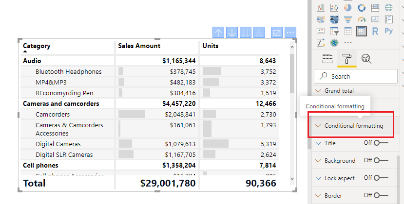
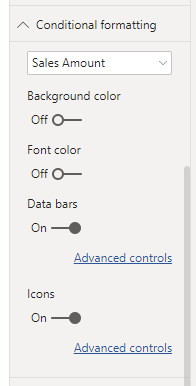
So what does this mean? Well, now you have a new Conditional Formatting box found in the settings of the Table and the Matrix properties. To use a built in Icon from Power BI. Create either a table or a Matrix visual with some data.
Select the visual and adjust it’s properties by clicking on the Paint Roller and opening the Conditional Formatting window.
Scroll down until you see the toggle button for Icons. Turn the Icons On.
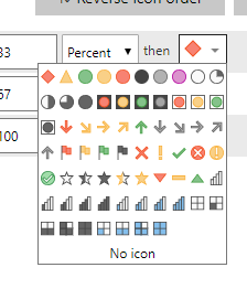
Click on the Advanced Controls to set the properties of the icons based on the data properties. This type of dialog box should look familiar as it is similar to the previous boxes for conditional formatting. Opening this window shows Icons for each Rule in the list. To adjust an icon Click on the Drop DownArrow next to the icon you wish to change. There are multiple icons to choose from.
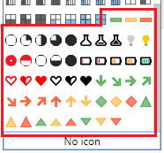
There are limited selections by default, but you can enhance this by adding your own icons with the custom Json theme files. At PowerBI.tips we love our theme files. They make using standard settings so much easier.
Loading the Custom Icons
For starters we have already done the hard work of creating an additional 50 icons for you to use in your reports. Download the Icon Theme File Here
Update: Special thanks to Reid Havens from Havens Consulting for contributing extra icons to this Icon Set.
Unzip the downloaded file to find the PowerBITips Icons v1.json file
Navigate to the Home ribbon in Power BI Desktop
Click on the Switch Theme button
Select the list item Import Theme from the drop down menu
The open file dialog box will open. Select the PowerBITips Icons v1.json file that you downloaded earlier.
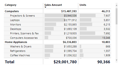
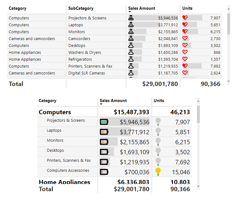
Boom, and just like that you have loaded your new icons. Now you can return to the icons for your table or matrix and adjust until your heart is content.
Here is a sample of a table and a matrix with some custom icons applied:
Update 2019/08/06: When publishing the Power BI file to the PowerBI.com service, the fill colors for the shapes need to have a %23 instead of a # (HASH) infront of the HEX codes. Thus, the format should look like fill=’%23FF0000′ instead of fill=’#FF0000′
If you like the content from PowerBI.Tips please follow us on all the social outlets. Stay up to date on all the latest features and free tutorials. Subscribe to our YouTube Channel. Or follow us on the social channels, Twitter and LinkedIn where we will post all the announcements for new tutorials and content.
Introducing our PowerBI.tips SWAG store. Check out all the fun PowerBI.tips clothing and products:
Check out the new Merch!
Hasta La Vista Data
Go Ahead Make My Data
PBIX Hat
Manage Consent
To provide the best experiences, we use technologies like cookies to store and/or access device information. Consenting to these technologies will allow us to process data such as browsing behavior or unique IDs on this site. Not consenting or withdrawing consent, may adversely affect certain features and functions.
Functional
Always active
The technical storage or access is strictly necessary for the legitimate purpose of enabling the use of a specific service explicitly requested by the subscriber or user, or for the sole purpose of carrying out the transmission of a communication over an electronic communications network.
Preferences
The technical storage or access is necessary for the legitimate purpose of storing preferences that are not requested by the subscriber or user.
Statistics
The technical storage or access that is used exclusively for statistical purposes.The technical storage or access that is used exclusively for anonymous statistical purposes. Without a subpoena, voluntary compliance on the part of your Internet Service Provider, or additional records from a third party, information stored or retrieved for this purpose alone cannot usually be used to identify you.
Marketing
The technical storage or access is required to create user profiles to send advertising, or to track the user on a website or across several websites for similar marketing purposes.